Visualizing Accelerometer Data in Python: A Case Study with the WitMotion WT901BLECL5.0

Using Python for vibration analysis and optimizing 3D printing parameters in silicon printing.

Introduction

In this article, I’ll walk you through my journey of collecting, visualizing, and analyzing accelerometer data from the WitMotion WT901BLECL5.0 sensor. The goal of this project is to use acceleration data to address vibration handling in 3D printer beds and optimize silicon printing parameters.

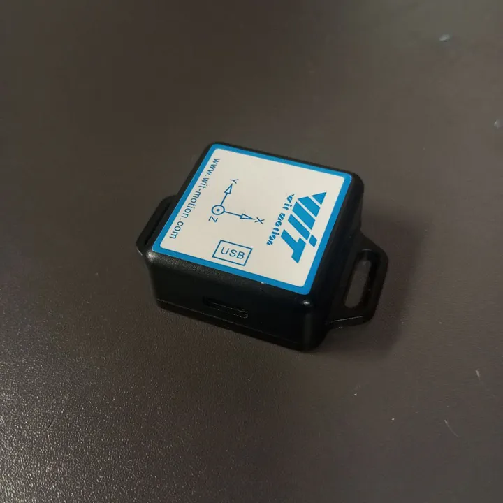
WitMotion WT901BLECL5.0 — Hardware & Software Overview

The Accelerometer

The WitMotion WT901BLECL5.0 is a versatile sensor capable of measuring:

• Acceleration
• Angular velocity
• Angles (roll, pitch, yaw)
• Temperature
• Magnetic field
• Humidity

Features of the Sensor

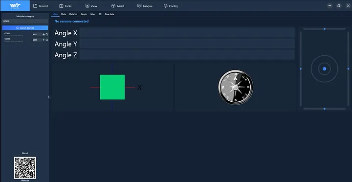
• Provides data via software with a built-in 3D visualization interface
• Records data and exports it as CSV for post-processing
• Supports Arduino, Python, Raspberry Pi, STM32, and ROS
• Includes an Android app for mobile data collection

Data Collection Process

For this experiment, I measured acceleration data on a 3D printer bed using an XYZ calibration cube print. This setup allowed me to observe the bed’s vibrations during printing.

Tools and Techniques

1. WitMotion Software

• Captured acceleration and orientation data
• Exported files in CSV format
• Explored roll, pitch, and yaw using the 3D visualization interface

2. Python Libraries

• Pandas – data cleaning and manipulation
• Matplotlib – visualization and plotting

3. Dataset Creation

Collected the following data types:

• Acceleration
• Angles
• Angular velocity
• Temperature
• Magnetic field

This resulted in a comprehensive dataset for analysis and potential future machine learning tasks.

Data Visualization in Python

To visualize the data, I wrote a Python script using Pandas and Matplotlib to generate time-series plots for angles, acceleration, angular velocity, magnetic field, temperature, and quaternions.

Python Code Snippet

import pandas as pd
import matplotlib.pyplot as plt

# Reload the uploaded data
file_path = 'C:/filepath/data.csv'
data = pd.read_csv(file_path)

# Clean the Time column
data['Time'] = data['Time'].str.strip()

# Define reference time
reference_time_str = "19:15:21.501"
reference_time = pd.to_datetime(reference_time_str, format='%H:%M:%S.%f')

# Convert 'Time' column to datetime and calculate time difference
data['Time'] = pd.to_datetime(data['Time'], format='%H:%M:%S.%f', errors='coerce')
data['Time Difference (s)'] = (data['Time'] - reference_time).dt.total_seconds()

print(data.columns)

# Define plotting function
def plot_data(subplot_titles, columns, title):
    fig, axes = plt.subplots(len(columns), 1, figsize=(10, 6), sharex=True)
    fig.suptitle(title, fontsize=16)
    for i, col in enumerate(columns):
        axes[i].plot(data['Time Difference (s)'], data[col], label=col, linewidth=1)
        axes[i].set_ylabel(col)
        axes[i].grid()
        axes[i].legend()
    axes[-1].set_xlabel('Time Difference (s)')
    plt.tight_layout()
    plt.subplots_adjust(top=0.9)
    plt.show()

# Plot angles
plot_data(
    ['Angle X(°)', 'Angle Y(°)', 'Angle Z(°)'],
    ['Angle X(°)', 'Angle Y(°)', 'Angle Z(°)'],
    'Angles (X, Y, Z)'
)

# Plot acceleration
plot_data(
    ['Acceleration X(g)', 'Acceleration Y(g)', 'Acceleration Z(g)'],
    ['Acceleration X(g)', 'Acceleration Y(g)', 'Acceleration Z(g)'],
    'Acceleration (X, Y, Z)'
)

# Plot angular velocity
plot_data(
    ['Angular velocity X(°/s)', 'Angular velocity Y(°/s)', 'Angular velocity Z(°/s)'],
    ['Angular velocity X(°/s)', 'Angular velocity Y(°/s)', 'Angular velocity Z(°/s)'],
    'Angular Velocity (X, Y, Z)'
)

# Plot magnetic field
plot_data(
    ['Magnetic field X(ʯt)', 'Magnetic field Y(ʯt)', 'Magnetic field Z(ʯt)'],
    ['Magnetic field X(ʯt)', 'Magnetic field Y(ʯt)', 'Magnetic field Z(ʯt)'],
    'Magnetic Field (X, Y, Z)'
)

# Plot temperature
plt.figure(figsize=(10, 4))
plt.plot(data['Time Difference (s)'], data['Temperature(℃)'], label='Temperature(℃)', linewidth=1)
plt.title('Temperature (℃)')
plt.xlabel('Time Difference (s)')
plt.ylabel('Temperature (℃)')
plt.grid()
plt.legend()
plt.show()

# Plot quaternions
plot_data(
    ['Quaternions 0()', 'Quaternions 1()', 'Quaternions 2()', 'Quaternions 3()'],
    ['Quaternions 0()', 'Quaternions 1()', 'Quaternions 2()', 'Quaternions 3()'],
    'Quaternions (0, 1, 2, 3)'
)

Read full article